Dashboard with Elastic sample data
Elastic provides sample data that can be installed under 'Integrations → Sample data → Other sample data sets'. The examples from "Sample eCommerce orders" are used in the following example. The example can be reproduced with this data.
Dashboard as a template
Data from the eCommerce example has been displayed in the dashboard in a tag cloud, a line chart, two bar charts and two gauge panels (level charts). The gauge panels show the data of individual customers from the eCommerce file via filters. The tag cloud panel with 25 tags and the panel with the line graph were created as "Legacy → Aggregation based" panels and then converted to Kibana Lens panels, the other panels were defined directly with Kibana Lens. The dashboard looks like this:
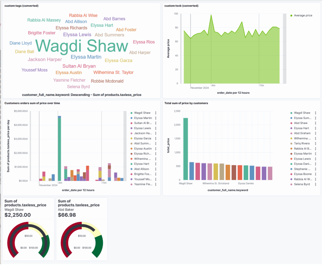
This example dashboard has then been exported to the blog_beispiel5.ndjson file.
Input file with variables
In the input file blog_beispiel5_vars.json some variables are defined again for the time being.
{
    "tag_cloud": {
        "title": "Customers with highest turnover",
        "number": 30
    },
    "area": {
        "title": "Average price of orders over time"
    },
    "bars_stacked": {
        "title": "Total cost of orders by customer over time"
    },
    "bars": {
        "title": "Total revenue per customer"
    },
    "gauge": {
        "height": 10,
        "width": 8
    },
    "dashboard_title": "generated_dashboard_blog_example5"
}
A title is again defined for the dashboard. Only different titles are set for the first 4 graphics and the number of tags is changed for the tag cloud and the size of the gauge panel is specified. These are all trivial adjustments, but they show how such a dashboard can be customised and regenerated with variables. This can then be expanded further if required.
Inserting jinja2 elements
The blog_beispiel5.j2 file has been reshaped so that it can be customised more easily. For the tag cloud panel, the title and the number of tags are inserted as follows:
"panelsJSON": "[{\"type\":\"lens\",
--------->\"gridData\":{\"x\":0,
--------->\"y\":0,
--------->\"w\":24,
--------->\"h\":15,
--------->\"i\":\"7338d1e1-501e-4084-8d8a-5b7593a87e66\"},
--------->\"panelIndex\":\"7338d1e1-501e-4084-8d8a-5b7593a87e66\",
--------->\"embeddableConfig\":{\"attributes\":{\"title\":\"{{ tag_cloud.title }}\",
--------->\"visualizationType\":\"lnsTagcloud\",
--------->\"type\":\"lens\",
--------->\"references\":[{\"type\":\"index-pattern\",
--------->\"id\":\"ff959d40-b880-11e8-a6d9-e546fe2bba5f\",
--------->\"name\":\"indexpattern-datasource-layer-83a576c3-0e7c-4f46-8284-f87ab836f522\"}],
--------->\"state\":{\"visualization\":{\"layerId\":\"83a576c3-0e7c-4f46-8284-f87ab836f522\",
--------->\"tagAccessor\":\"8ff218c8-cd38-42a9-90bf-06ba8c0543a1\",
--------->\"valueAccessor\":\"d0227fac-22a7-4277-aa2e-cabe22f58736\",
--------->\"maxFontSize\":72,
--------->\"minFontSize\":18,
--------->\"orientation\":\"single\",
--------->\"showLabel\":true,
--------->\"colorMapping\":{\"assignments\":[],
--------->\"specialAssignments\":[{\"rule\":{\"type\":\"other\"},
--------->\"color\":{\"type\":\"loop\"},
--------->\"touched\":false}],
--------->\"paletteId\":\"eui_amsterdam_color_blind\",
--------->\"colorMode\":{\"type\":\"categorical\"}},
--------->\"layerType\":\"data\",
--------->\"palette\":{\"name\":\"default\",
--------->\"type\":\"palette\"}},
--------->\"query\":{\"query\":\"\",
--------->\"language\":\"kuery\"},
--------->\"filters\":[],
--------->\"datasourceStates\":{\"formBased\":{\"layers\":{\"83a576c3-0e7c-4f46-8284-f87ab836f522\":{\"ignoreGlobalFilters\":false,
--------->\"columns\":{\"8ff218c8-cd38-42a9-90bf-06ba8c0543a1\":{\"label\":\"customer_full_name.keyword: Descending\",
--------->\"dataType\":\"string\",
--------->\"operationType\":\"terms\",
--------->\"scale\":\"ordinal\",
--------->\"sourceField\":\"customer_full_name.keyword\",
--------->\"isBucketed\":true,
--------->\"params\":{\"size\":{{ tag_cloud.anzahl }},
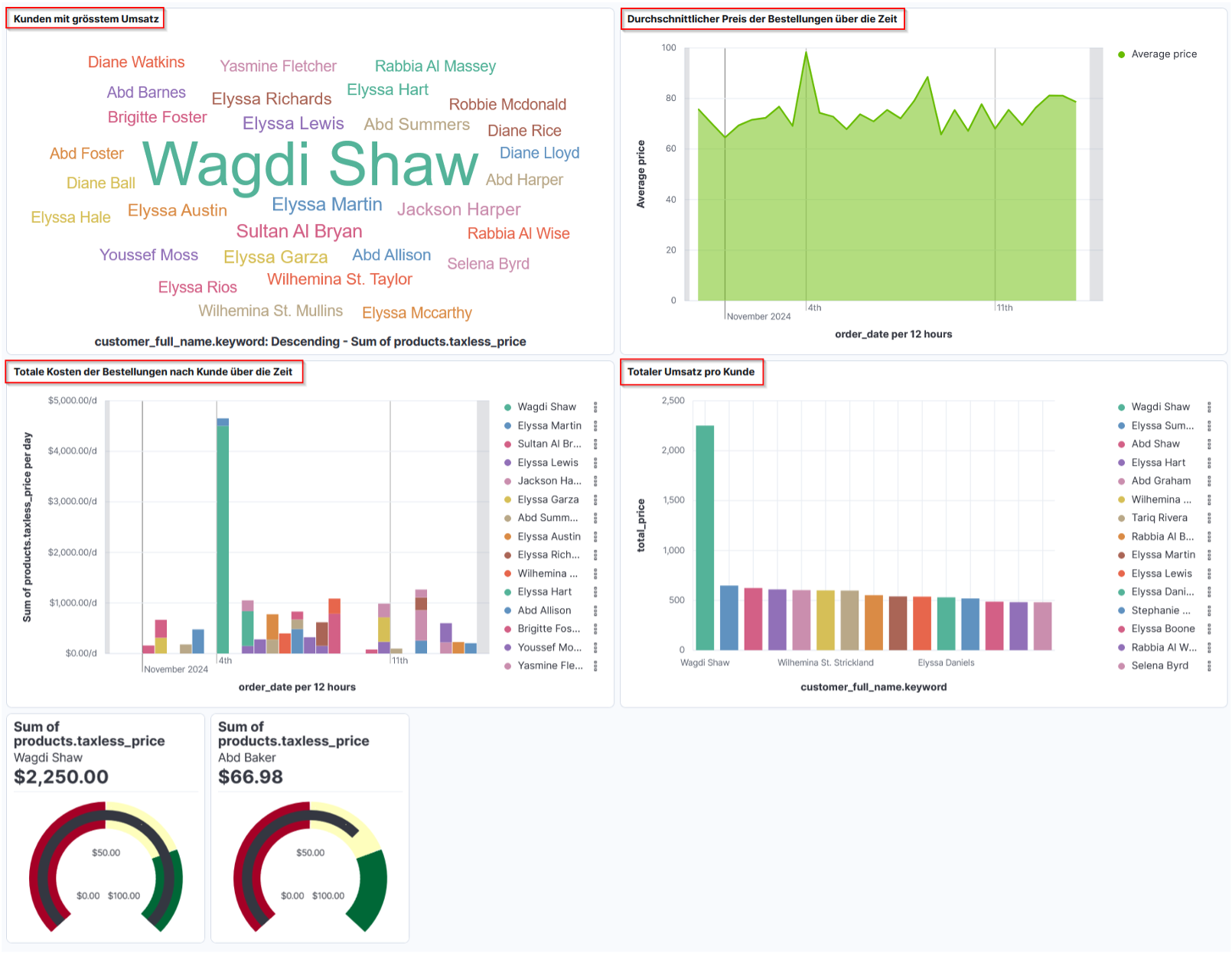
--------->\"orderBy\":{\"type\":\"column\",The dashboard ID is deleted again so that Kibana generates a new, unique dashboard ID during import.
    "created_at": "2024-12-11T16:21:16.255Z",
 "id": "24248d69-cca9-4e52-be60-bd2fa96d24ac",
The dashboard generated with the template and the above input file then looks as follows, whereby the tag cloud panel now displays 30 tags and the titles of the panels are customised (framed in red in the screenshot):
Input file for a flexible number of gauge panels
To make example 5 a little more interesting, the input file is supplemented with variables for several gauge panels. These should be arranged in rows and columns like the markdown panels in the previous example and they should display information for different customers from the eCommerce sample data.
    "tag_cloud": {
        "title": "Customers with highest turnover",
        "number": 30
    },
    "area": {
        "title": "Average price of orders over time"
    },
    "bars_stacked": {
        "title": "Total cost of orders by customer over time"
    },
    "bars": {
        "title": "Total revenue per customer"
    },
    "gauge": {
        "height": 10,
        "width": 8,
        "columns": 6,
        "number": 20
    },
    }, "name": [
        "Wagdi Shaw",
        "Elyssa Summers",
        "Abd Shaw",
        "Elyssa Hart",
        "Abd Graham",
        "Wilhemina St Strickland",
        "Tariq Rivera",
        "Rabbia Al Baker",
        "Elyssa Martin",
        "Elyssa Lewis",
        "Elyssa Daniels."
        // etc. ...
        "Elyssa Hale",
        "Abd Burton",
        "Sultan Al Marshall",
        "Betty Morrison",
        "Mary Hampton",
        "Elyssa Rowe",
        "Elyssa Austin"
    ],
    "dashboard_title": "generated_dashboard_blog_example5"
}
The array with the names of customers from eCommerce can be used for the filters and labelling of the gauge panels.
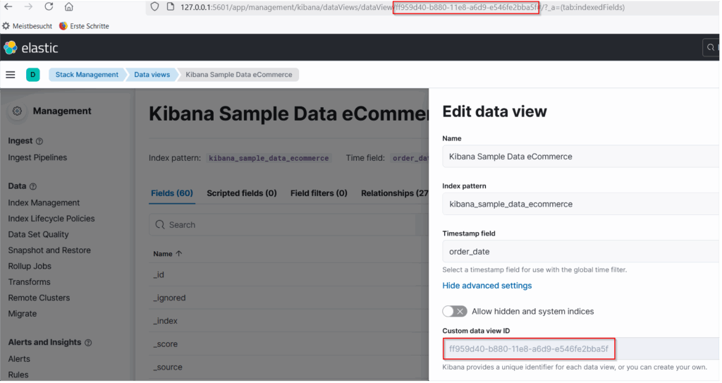
Data View IDs
DataView IDs are used in Kibana for references to the data. In the ndjson files, the former name Index patters is used. The DataView IDs are usually already present in the ndjson template and can simply be reused. Otherwise, you can find the DataView IDs under "Stack Management→DataViews". There you select the DataView, click on "Edit" and "Show advanced settings" and the DataView ID is then displayed. The ID is also part of the url:
References and panel IDs
Unlike the examples with the Markdown panels, Example 5 uses data stored in Elastic that is accessed from the dashboard. For this purpose, references and ids are defined in the dashboard towards the end of the ndjson file and referenced in the "references" array in the gauge panels, for example.
Some documentation can be found under the following links:
References
References (references) are regular saved object references forming a graph of saved objects which depend on each other. For the Lens case, these references can be annotation groups or data views (called type: "index-pattern" in code), referencing permanent data views which are used in the current Lens visualisation. Often there is just a single data view in use, but it's possible to use multiple data views for multiple layers in a Lens xy chart. The id of a reference needs to be the saved object id of the referenced data view (see the "Handling data views" section below). The name of the reference is comprised out of multiple parts used to map the data view to the correct layer : indexpattern-datasource-layer-. Even if multiple layers are using the same data view, there has to be one reference per layer (all pointing to the same data view id). References array can be empty in case of adhoc dataviews (see section below).
references array
Objects with name, id, and type properties that describe the other saved objects that this object references. Use name in attributes to refer to the other saved object, but never the idwhich can update automatically during migrations or import and export.
In the exported dashboard template, the definition of the references looks like this, for example:
    "references": [
        {
            "id": "ff959d40-b880-11e8-a6d9-e546fe2bba5f",
            "name": "7338d1e1-501e-4084-8d8a-5b7593a87e66:indexpattern-datasource-layer-83a576c3-0e7c-4f46-8284-f87ab836f522",
            "type": "index-pattern"
        },
//... ...
        {
            "id": "ff959d40-b880-11e8-a6d9-e546fe2bba5f",
            "name": "1400e794-2571-4b4a-b78b-2d5aab20263b:indexpattern-datasource-layer-38148eb9-48c3-40ac-8090-011abf2cdefe",
            "type": "index-pattern"
        },
        {
            "id": "ff959d40-b880-11e8-a6d9-e546fe2bba5f",
            "name": "1400e794-2571-4b4a-b78b-2d5aab20263b:08984911-134f-4ff2-8c1d-bf86d034351c",
            "type": "index-pattern"
        }
    ],
The entries with
"name": "1400e794-2571-4b4a-b78b-2d5aab20263bare those that are referenced in the one gauge panel. This is where the "name" as "panelIndex" and as a component "i" in "gridData". This allows you to find these entries in the reference array. The other entries there belong to the other panels. "id" is the DataView ID for the eCommerce sample data everywhere, which is referenced from all panels.
If several gauge panels are to be defined in the dashboard, they must all have a unique panel index. There are apparently no major specifications for the format of the panel indices, so you are fairly free to choose unique values. The panel indices must be defined in the gauge panel definitions and must match the references in the array.
Inserting jinja2 elements
The definitions of the gauge panels are generated in a loop like those for the Markdown panels in example4.j2. The panel index is simply "gauge_panel_nri", where "i" is a sequence number. In this way, the indices can be easily generated for the panels and the references in two independent loops.
The most important jinja2 elements in the definition of the gauge panels in blog_beisiel5.j2 are then:
--------->{% set global = namespace(row = 0) %}{% for i in range(0, gauge.number) %}{\"type\":\"lens\",
--------->\"gridData\":{\"x\":{{ (i) % gauge.columns * gauge.width }},
--------->\"y\":{{ 30 + gauge.height * global.row }}{% if (i + 1) % gauge.columns == 0 %}{% set global.row = global.row + 1 %}{% endif %},
--------->\"w\":{{ gauge.width }},
--------->\"h\":{{ gauge.height }},
--------->\"i\":\"gauge_panel_nr{{ i }}\"},
--------->\"panelIndex\":\"gauge_panel_nr{{ i }}\",
--------->\"embeddableConfig\":{\"attributes\":{\"title\":\"Gauge visualization\",
--------->\"visualizationType\":\"lnsGauge\",
--------->\"type\":\"lens\",
--------->\"references\":[{\"type\":\"index-pattern\",
--------->\"id\":\"ff959d40-b880-11e8-a6d9-e546fe2bba5f\",
--------->\"name\":\"indexpattern-datasource-layer-38148eb9-48c3-40ac-8090-011abf2cdefe\"}],
--------->\"state\":{\"visualization\":{\"shape\":\"arc\",
--------->\"layerId\":\"38148eb9-48c3-40ac-8090-011abf2cdefe\",
--------->\"layerType\":\"data\",
--------->\"ticksPosition\":\"auto\",
--------->\"labelMajorMode\":\"auto\",
--------->\"metricAccessor\":\"e4f872bd-8510-456b-ac48-8da24c92b19d\",
--------->\"colorMode\":\"palette\",
--------->\"percentageMode\":false,
--------->\"palette\":{\"name\":\"custom\",
--------->\"params\":{\"maxSteps\":5,
--------->\"name\":\"custom\",
--------->\"progression\":\"fixed\",
--------->\"rangeMax\":100,
--------->\"rangeMin\":0,
--------->\"rangeType\":\"number\",
--------->\"reverse\":false,
--------->\"continuity\":\"none\",
--------->\"colorStops\":[{\"color\":\"#A50026\",
--------->\"stop\":0},
--------->{\"color\":\"#FEFEBD\",
--------->\"stop\":50},
--------->{\"color\":\"#006837\",
--------->\"stop\":75}],
--------->\"stops\":[{\"color\":\"#A50026\",
--------->\"stop\":50},
--------->{\"color\":\"#FEFEBD\",
--------->\"stop\":75},
--------->{\"color\":\"#006837\",
--------->\"stop\":100}],
--------->\"steps\":5},
--------->\"type\":\"palette\"},
--------->\"minAccessor\":\"4399d773-95c6-4ecb-bc1b-a26a9d9f0d09\",
--------->\"maxAccessor\":\"9a3f8db0-a822-4627-9906-8fab5bf235df\",
--------->\"labelMinor\":\"{{ name[i] }}\"},
--------->\"query\":{\"query\":\"customer_full_name.keyword : \\\"{{ name[i] }}\\\"  \",
--------->\"language\":\"kuery\"},
--------->\"filters\":[{\"meta\":{\"alias\":null,
--------->\"disabled\":false,
--------->\"index\":\"5c0dea8b-d51a-4f34-8240-520a78d12164\",
--------->\"key\":\"products.taxless_price\",
--------->\"negate\":false,
--------->\"type\":\"exists\",
--------->\"value\":\"exists\"},
--------->\"query\":{\"exists\":{\"field\":\"products.taxless_price\"}},
//... ...
--------->\"enhancements\":{},
--------->\"hidePanelTitles\":true},
--------->\"title\":\"Gauge visualisation\"}{% if loop.index != loop.length %},{% endif %}{% endfor %}]",
At the beginning and end are the specifications for the loop, whereby at the end it must be checked again whether a comma is necessary or whether the last element of the array has been reached. The calculation of the position of the panels is done analogue to example 4.
In addition, the name from the array with the customer names is defined as a label and specified in the filter query.
The two definitions for the panel indices are important.
--------->\"i\":\"gauge_panel_nr{{ i }}\"},
--------->\"panelIndex\":\"gauge_panel_nr{{ i }}\",
In addition, the references for all gauge panels must be generated in a loop below.
{
"id": "ff959d40-b880-11e8-a6d9-e546fe2bba5f",
"name": "51c3912f-6d82-4be5-82e4-31a6549d9df4:indexpattern-datasource-layer-446d03ef-469d-419a-90ab-40632cd777f5",
"type": "index-pattern"
},
{% for i in range(0, gauge.number) %}{
"id": "ff959d40-b880-11e8-a6d9-e546fe2bba5f",
"name": "gauge_panel_nr{{ i }}:indexpattern-datasource-layer-38148eb9-48c3-40ac-8090-011abf2cdefe",
"type": "index-pattern"
},{% endfor %}
{
"id": "ff959d40-b880-11e8-a6d9-e546fe2bba5f",
"name": "gauge_panel_nr0:08984911-134f-4ff2-8c1d-bf86d034351c",
"type": "index-pattern"
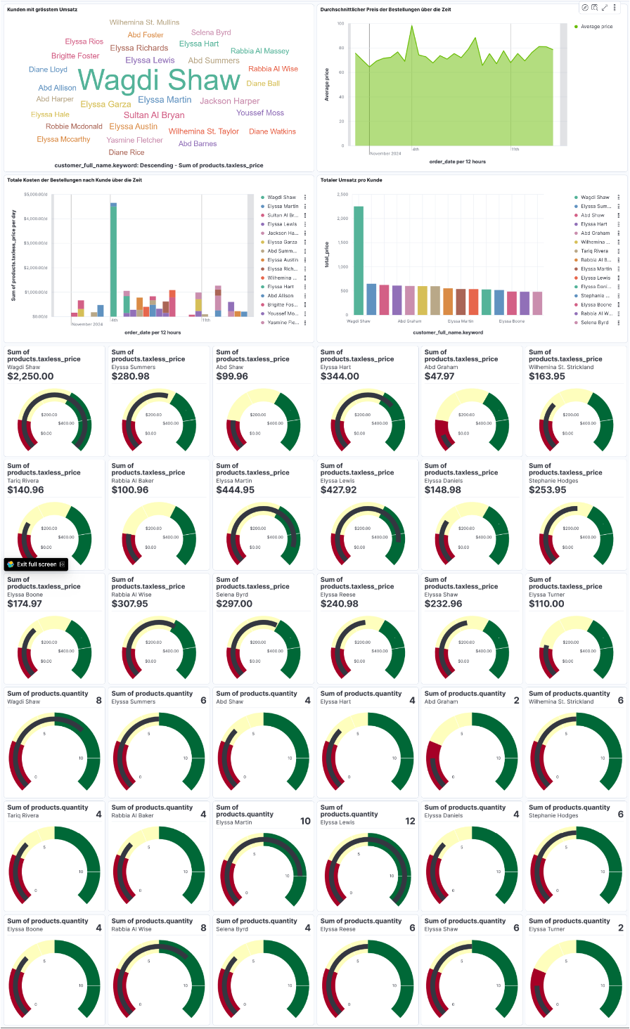
}The command
jinjanate blog_beispiel5.j2 blog_beispiel5_vars.json -o generated_dashboard_blog_beispiel5.ndjsonnow generates the following dashboard, in which the gauge panels are repeated and arranged regularly in 6 columns:
Variant with gauge panels for different metrics
As a further variant of example 5, I have generated gauge panels for two metrics and defined the limits for the colours and the maximum values in the gauge panels using variables in the input file. If only one metric is specified, the previous dashboard can also be generated.
Input file with two metrics for the gauge panels
The following part of the input file has been adapted, whereby arrays have been used for each of the entries.
    "gauge": {
        "height": 10,
        "width": 8,
        "columns": 6,
        "number": 18,
        "query_fields": [
            "products.taxless_price",
            "products.quantity"
        ],
        "range_max" : [500, 12],
        "colour_start" : [[0, 100, 300],
                                        [0,3,6]],
        "colour_stop" : [[100, 300, 500],
                                       [3,6,12]]
    },
    "name": [
        "Wagdi Shaw",
        "Elyssa Summers",
Inserting jinja2 elements
Two nested loops are now required here, one via the metrics and within this loop one each via the number of desired gauge panels.
To help you, here are the important parts of the json file before it was reformatted to blog_beispiel5.j2:
--------->{% set global = namespace(row = 0) %}{% for field in gauge.query_fields %}{% set outer_loop = loop %}{% for i in range(0, gauge.number) %}{\"type\":\"lens\",
--------->\"gridData\":{\"x\":{{ (i + ( outer_loop.index0 * gauge.number ) ) % gauge.columns * gauge.width }},
--------->\"y\":{{ 30 + gauge.height * global.row }}{% if (i + 1 + ( outer_loop.index0 * gauge.number ) ) % gauge.columns == 0 %}{% set global.row = global.row + 1 %}{% endif %},
--------->\"w\":{{ gauge.width }},
--------->\"h\":{{ gauge.height }},
--------->\"i\":\"gauge_panel_nr{{ i + ( outer_loop.index0 * gauge.number ) }}\"},
--------->\"panelIndex\":\"gauge_panel_nr{{ i + ( outer_loop.index0 * gauge.number ) }}\",
--------->\"embeddableConfig\":{\"attributes\":{\"title\":\"Gauge visualization\",
//... ...
--------->\"rangeMax\":{{ gauge.range_max[outer_loop.index0] }},
--------->\"rangeMin\":0,
--------->\"rangeType\":\"number\",
--------->\"reverse\":false,
--------->\"continuity\":\"none\",
--------->\"colorStops\":[{\"color\":\"#A50026\",
--------->\"stop\":{{ gauge.color_start[outer_loop.index0][0] }}},
--------->{\"color\":\"#FEFEBD\",
--------->\"stop\":{{ gauge.color_start[outer_loop.index0][1] }}},
--------->{\"color\":\"#006837\",
--------->\"stop\":{{ gauge.color_start[outer_loop.index0][2] }}}],
--------->\"stops\":[{\"color\":\"#A50026\",
--------->\"stop\":{{ gauge.color_stop[outer_loop.index0][0] }}},
--------->{\"color\":\"#FEFEBD\",
--------->\"stop\":{{ gauge.color_stop[outer_loop.index0][1] }}},
--------->{\"color\":\"#006837\",
--------->\"stop\":{{ gauge.color_stop[outer_loop.index0][2] }}}],
--------->\"steps\":5},
//... ...
--------->\"9a3f8db0-a822-4627-9906-8fab5bf235df\":{\"label\":\"Static value: {{ gauge.range_max[outer_loop.index0] }}\",
--------->\"dataType\":\"number\",
--------->\"operationType\":\"static_value\",
--------->\"isStaticValue\":true,
--------->\"isBucketed\":false,
--------->\"scale\":\"ratio\",
--------->\"params\":{\"value\":\"{{ gauge.range_max[outer_loop.index0] }}\"},
//... ...
--------->\"title\":\"Gauge visualisation\"}{% if outer_loop.index != outer_loop.length or loop.index != loop.length %},{% endif %}{% endfor %}{% endfor %}]",
The generated dashboard with the gauge panels for the two different metrics then looks as follows:
Further ideas
The aim of this blog series is to introduce the principle of generating dashboards with jinja2 templates. Many other ideas for automation can be implemented in the same way, including in other areas.
Automation can be extended with shell scripts or scripts in other scripting languages. For example, several dashboards can be generated in one script or dashboards for different environments or customers can be generated in a loop.
Several dashboards can also be written to a single ndjson file.
The import of dashboards into Kibana via REST interface can also be inserted into the same script after the generation of dashboards. The documentation can be found here:
- https://www.elastic.co/docs/api/doc/kibana/operation/operation-importsavedobjectsdefault
- https://www.elastic.co/docs/api/doc/kibana/operation/operation-resolveimporterrors
Conclusion
Kibana dashboards can be generated flexibly with the ideas and tools presented. Unfortunately, there is no reference documentation for the format of the ndjson files used when exporting and importing dashboards and other saved objects. This sometimes requires a little imagination and testing for the actual implementation. However, the procedure quickly pays off if several similar dashboards are needed.
The same approach to automation can be used not only in the Elastic Stack but with many other software packages.
Register without hesitation for a free consultation at Swissmakers to find out how we can support you in the areas of automation and Elastic.